image layer tutorial

Welcome to the tutorial on the napari Image layer!

This tutorial assumes you have already installed napari, know how to launch the viewer, and are familiar with its layout. For help with installation see our installation tutorial. For help getting started with the viewer see our getting started tutorial. For help understanding the organisation of the viewer, including things like the layers list, the layer properties widgets, the layer control panels, and the dimension sliders see our napari viewer tutorial.

This tutorial will teach you about the napari Image layer, including the types of images that can be displayed, and how to set properties like the contrast, opacity, colormaps and blending mode. At the end of the tutorial you should understand how to add and manipulate a variety of different types of images both from the GUI and from the console.

a simple example

You can create a new viewer and add an image in one go using the napari.view_image method, or if you already have an existing viewer, you can add an image to it using viewer.add_image. The api of both methods is the same. In these examples we’ll mainly use view_image.

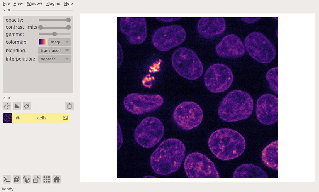
A simple example of viewing an image is as follows:

%gui qt  # we need to start the Qt event loop before importing napari

ERROR:root:Invalid GUI request 'qt # we need to start the Qt event loop before importing napari', valid ones are:dict_keys(['inline', 'nbagg', 'notebook', 'ipympl', 'widget', None, 'qt4', 'qt', 'qt5', 'wx', 'tk', 'gtk', 'gtk3', 'osx', 'asyncio'])

import napari
from skimage import data

cells = data.cells3d()[30, 1]  # grab some data
viewer = napari.view_image(cells, colormap='magma')

WARNING: QStandardPaths: XDG_RUNTIME_DIR not set, defaulting to '/tmp/runtime-runner'

WARNING:vispy:QStandardPaths: XDG_RUNTIME_DIR not set, defaulting to '/tmp/runtime-runner'

from napari.utils import nbscreenshot

nbscreenshot(viewer)

arguments of view_image and add_image

Both view_image and add_image have the following doc strings:

napari.view_image?

image data and numpy-like arrays

napari can take any numpy-like array as input for its image layer. A numpy-like array can just be a numpy array, a dask array, an xarray, a zarr array, or any other object that you can index into and when you call np.asarray on it you get back a numpy array.

The great thing about napari support array-like objects is that you get to keep on using your favorite array libraries without worrying about any conversions as we’ll handle all of that for you.

napari will also wait until just before it displays data onto the screen to actually generate a numpy array from your data, and so if you’re using a library like dask or zarr that supports lazy loading and lazy evaluation, we won’t force you load or compute on data that you’re not looking at. This enables napari to seamlessly browse enormous datasets that are loaded in the right way. For example, here we are browsing over 100GB of lattice lightsheet data stored in a zarr file:

image pyramids

For exceptionally large datasets napari supports image pyramids. An image pyramid is a list of arrays, where each array is downsampling of the previous array in the list, so that you end up with images of successively smaller and smaller shapes. A standard image pyramid might have a 2x downsampling at each level, but napari can support any type of pyramid as long as the shapes are getting smaller each time.

Image pyramids are especially useful for incredibly large 2D images when viewed in 2D or incredibly large 3D images when viewed in 3D. For example this ~100k x 200k pixel pathology image consists of 10 pyramid levels and can be easily browsed as at each moment in time we only load the level of the pyramid and the part of the image that needs to be displayed:

This example had precomputed image pyramids stored in a zarr file, which is best for performance. If, however you don’t have a precomputed pyramid but try and show a exceptionally large image napari will try and compute pyramids for you unless you tell it not too.

You can use the is_pyramid keyword argument to specify if your data is an image pyramid or not. If you don’t provide this value, then will try and guess whether your data is or needs to be an image pyramid.

3D rendering of images

All our layers can be rendered in both 2D and 3D mode, and one of our viewer buttons can toggle between each mode. The number of dimensions sliders will be 2 or 3 less than the total number of dimensions of the layer, allowing you to browse volumetric timeseries data and other high dimensional data. See for example these cells undergoing mitosis in this volumetric timeseries:

viewing rgb vs luminance (grayscale) images

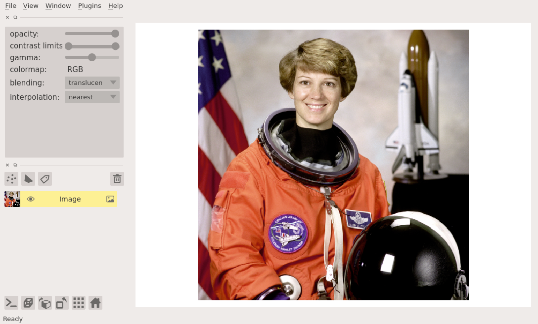
In this example we explicitly set the rgb keyword to be True because we know we are working with an rgb image:

import napari
from skimage import data

viewer = napari.view_image(data.astronaut(), rgb=True)

from napari.utils import nbscreenshot

nbscreenshot(viewer)

If we had left that keyword argument out napari would have successfully guessed that we were trying to show an rgb or rgba image because the final dimension was 3 or 4. If you have a luminance image where the last dimension is 3 or 4 you can set the rgb property to False so napari handles the image correctly.

rgb data must either be uint8, corresponding to values between 0 and 255, or float and between 0 and 1. If the values are float and outside the 0 to 1 range they will be clipped.

working with colormaps

napari supports any colormap that is created with vispy.color.Colormap. We provide access to some standard colormaps that you can set using a string of their name.

These include:

• PiYG

• blue

• cyan

• gist_earth

• gray

• green

• hsv

• inferno

• magma

• magenta

• plasma

• red

• turbo

• twilight

• twilight_shifted

• yellow

• viridis

Passing any of these as follows:

viewer = napari.view_image(data.moon(), colormap='red')

… will set the colormap of that image. You can also access the current colormap through the layer.colormap property which returns a tuple of the colormap name followed by the vispy colormap object. You can list all the available colormaps using layer.colormaps.

It is also possible to create your own colormaps using vispy’s vispy.color.Colormap object, see it’s full documentation here. Briefly, you can pass Colormap a list of length 3 or length 4 lists, corresponding to the rgb or rgba values at different points along the colormap.

For example, to make a diverging colormap that goes from red to blue through black, and color a random array you can do the following:

import napari
import numpy as np
from vispy.color import Colormap

cmap = Colormap([[1, 0, 0], [0, 0, 0], [0, 0, 1]])
image = np.random.random((100, 100))

viewer = napari.view_image(image, colormap=('diverging', cmap))

from napari.utils import nbscreenshot

nbscreenshot(viewer)

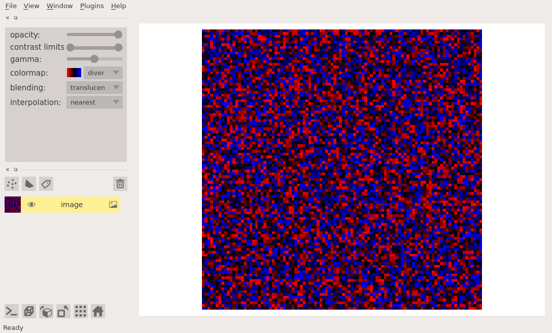
Note in this example how we passed the colormap keyword argument as a tuple containing both a name for our new custom colormap and the colormap itself. If we had only passed the colormap it would have been given a default name.

The named colormap now appears in the dropdown menu alongside a little thumbnail of the full range of the colormap.

adjusting contrast limits

Each image layer gets mapped through its colormap according to values called contrast limits. The contrast limits are a 2-tuple where the second value is larger than the first. The smaller contrast limit corresponds to the value of the image data that will get mapped to the color defined by 0 in the colormap. All values of image data smaller than this value will also get mapped to this color. The larger contrast limit corresponds to the value of the image data that will get mapped to the color defined by 1 in the colormap. All values of image data larger than this value will also get mapped to this color.

For example, you are looking at an image that has values between 0 and 100 with a standard gray colormap, and you set the contrast limits to (20, 75). Then all the pixels with values less than 20 will get mapped to black, the color corresponding to 0 in the colormap, and all pixels with values greater than 75 will get mapped to white, the color corresponding to 1 in the colormap. All other pixel values between 20 and 75 will get linearly mapped onto the range of colors between black and white.

In napari you can set the contrast limits when creating an Image layer or on an existing layer using the contrast_limits keyword argument or property, respectively.

import napari
from skimage import data

viewer = napari.view_image(data.moon(), name='moon')
viewer.layers['moon'].contrast_limits=(100, 175)

from napari.utils import nbscreenshot

nbscreenshot(viewer)

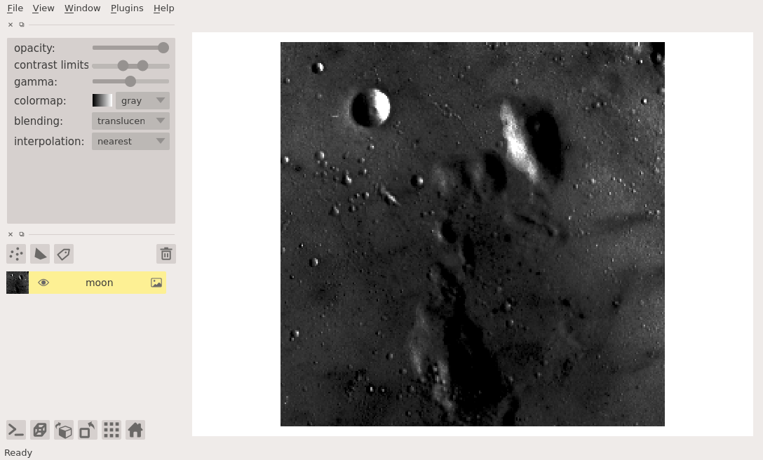
Because the contrast limits are defined by two values the corresponding slider has two handles, one the adjusts the smaller value, one that adjusts the larger value.

As of right now adjusting the contras limits has no effect for rgb data.

If no contrast limits are passed, then napari will compute them. If your data is small, then napari will just take the minimum and maximum values across your entire image. If your data is exceptionally large, this operation can be very time consuming and so if you have passed an image pyramid then napari will just use the top level of that pyramid, or it will use the minimum and maximum values across the top, middle, and bottom slices of your image. In general, if working with big images it is recommended you explicitly set the contrast limits if you can.

Currently if you pass contrast limits as a keyword argument to a layer then full extent of the contrast limits range slider will be set to those values.

layer visibility

All our layers support a visibility toggle that allows you to set the visible property of each layer. This property is located inside the layer widget in the layers list and is represented by an eye icon.

layer opacity

All our layers support an opacity slider and opacity property that allow you to adjust the layer opacity between 0, fully invisible and 1, fully visible.

blending layers

All our layers support three blending modes translucent, additive, and opaque that determine how the visuals for this layer get mixed with the visuals from the other layers.

An opaque layer renders all the other layers below it invisible and will fade to black as you decrease its opacity.

The translucent setting will cause the layer to blend with the layers below it if you decrease its opacity but will fully block those layers if its opacity is 1. This is a reasonable default, useful for many applications.

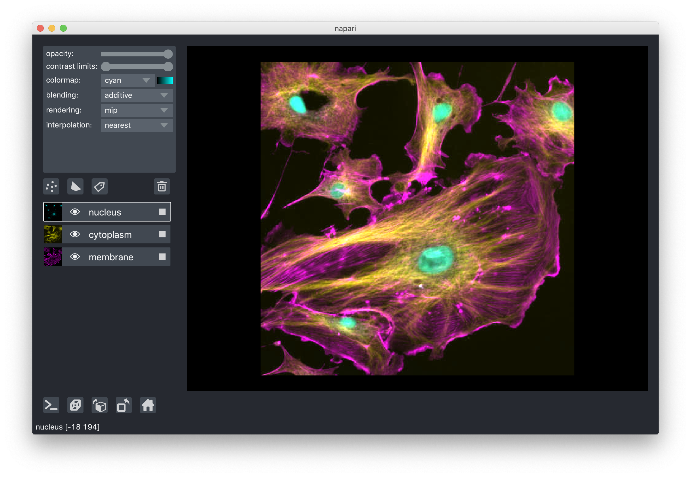
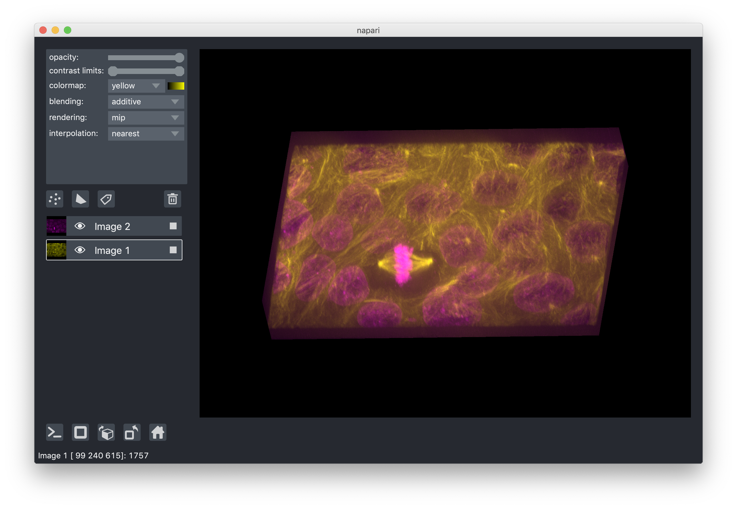
The final blending mode additive will cause the layer to blend with the layers below even when it has full opacity. This mode is especially useful for many cell biology applications where you have multiple different components of a cell labeled in different colors.

For example:

layer interpolation

We support a variety of interpolation modes when viewing 2D slices. In the default mode nearest each pixel is represented as a small square of specified size. As you zoom in you will eventually see each pixel. In other modes neighbouring pixels are blended together according to different functions, for example bicubic, which can lead to smoother looking images. For most scientific use-cases nearest is recommended because it does not introduce more artificial blurring. These modes have no effect when viewing 3D slices.

layer rendering

When viewing 3D slices, we support a variety of rendering modes. The default mode mip, or maximum intensity projection, will combine voxels at different distances from the camera according to a maximum intensity projection to create the 2D image that is then displayed on the screen. This mode works well for many biological images such as these cells growing in culture:

When viewing 2D slices the rendering mode has no effect.

naming layers

All our layers support a name property that can be set inside a text box inside the layer widget in the layers list. The name of each layer is forced into being unique so that you can use the name to index into viewer.layers to retrieve the layer object.

scaling layers

All our layers support a scale property and keyword argument that will rescale the layer multiplicatively according to the scale values (one for each dimension). This property can be particularly useful for viewing anisotropic volumes where the size of the voxel in the z dimension might be different then the size in the x and y dimensions.

translating layers

All our layers support a translate property and keyword argument that you can use to offset a layer relative to the other layers, which could be useful if you are trying to overlay two layers for image registration purposes.

layer metadata

All our layers also support a metadata property and keyword argument that you can use to store an arbitrary metadata dictionary on the layer.

next steps

Hopefully, this tutorial has given you a detailed understanding of the Image layer, including how to create one and control its properties. To learn more about some of the other layer types that napari supports checkout some more of our tutorials listed below. The labels layer tutorial is a great one to try next as labels layers are an extension of our image layers used for labeling regions of images.