surface layer tutorial¶

Welcome to the tutorial on the napari Surface layer!

This tutorial assumes you have already installed napari, know how to launch the viewer, and are familiar with its layout. For help with installation see our installation tutorial. For help getting started with the viewer see our getting started tutorial. For help understanding the organisation of the viewer, including things like the layers list, the layer properties widgets, the layer control panels, and the dimension sliders see our napari viewer tutorial.

This tutorial will teach you about the napari Surface layer, including how to display surface data and edit the properties of surfaces like the contrast, opacity, colormaps and blending mode. At the end of the tutorial you should understand how to add and manipulate surfaces both from the GUI and from the console.

The surface layer allows you to display a precomputed surface mesh that is defined by an NxD array of N vertices in D coordinates, an Mx3 integer array of the indices of the triangles making up the faces of the surface, and a length N list of values to associate with each vertex to use alongside a colormap.

a simple example¶

You can create a new viewer and add a surface in one go using the napari.view_surface method, or if you already have an existing viewer, you can add an image to it using viewer.add_surface. The api of both methods is the same. In these examples we’ll mainly use view_surface.

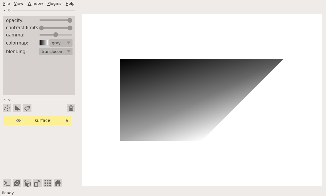
A simple example of viewing a surface is as follows:

%gui qt  # we need to start the Qt event loop before importing napari

ERROR:root:Invalid GUI request 'qt # we need to start the Qt event loop before importing napari', valid ones are:dict_keys(['inline', 'nbagg', 'notebook', 'ipympl', 'widget', None, 'qt4', 'qt', 'qt5', 'wx', 'tk', 'gtk', 'gtk3', 'osx', 'asyncio'])

import napari
import numpy as np

vertices = np.array([[0, 0], [0, 20], [10, 0], [10, 10]])
faces = np.array([[0, 1, 2], [1, 2, 3]])
values = np.linspace(0, 1, len(vertices))
surface = (vertices, faces, values)

viewer = napari.view_surface(surface)  # add the surface

WARNING: QStandardPaths: XDG_RUNTIME_DIR not set, defaulting to '/tmp/runtime-runner'

WARNING:vispy:QStandardPaths: XDG_RUNTIME_DIR not set, defaulting to '/tmp/runtime-runner'

from napari.utils import nbscreenshot

nbscreenshot(viewer)

arguments of view_surface and add_surface¶

Both view_surface and add_surface have the following doc strings:

napari.view_surface?

surface data¶

The data for a surface layer is defined by a 3-tuple of its vertices, faces, and vertex values. The vertices are an NxD array of N vertices in D coordinates. The faces are an Mx3 integer array of the indices of the triangles making up the faces of the surface. The vertex values are a length N list of values to associate with each vertex to use alongside a colormap. This 3-tuple is accessible through the layer.data property.

3D rendering of images¶

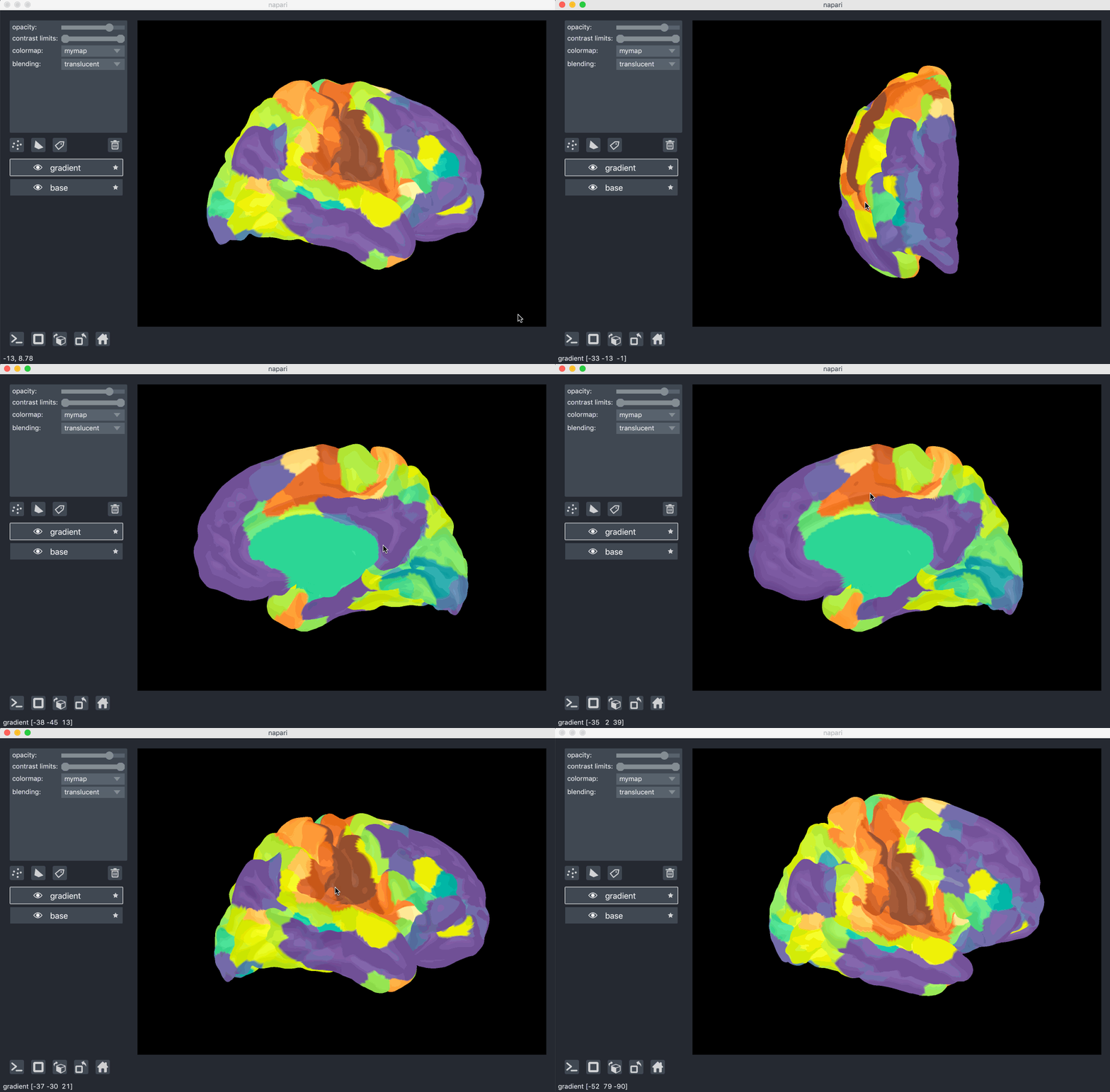
All our layers can be rendered in both 2D and 3D mode, and one of our viewer buttons can toggle between each mode. The number of dimensions sliders will be 2 or 3 less than the total number of dimensions of the layer. See for example these brain surfaces rendered in 3D:

image: brain surface

working with colormaps¶

The same colormaps available for the Image layer are also available for the Surface layer. napari supports any colormap that is created with vispy.color.Colormap. We provide access to some standard colormaps that you can set using a string of their name.

These include:

PiYG
blue
cyan
gist_earth
gray
green
hsv
inferno
magma
magenta
plasma
red
turbo
twilight
twilight_shifted
yellow
viridis

Passing any of these as follows as keyword arguments will set the colormap of that surface. You can also access the current colormap through the layer.colormap property which returns a tuple of the colormap name followed by the vispy colormap object. You can list all the available colormaps using layer.colormaps.

It is also possible to create your own colormaps using vispy’s vispy.color.Colormap object, see it’s full documentation here. For more detail see the image layer tutorial.

adjusting contrast limits¶

The vertex values of the surface layer get mapped through its colormap according to values called contrast limits. These are a 2-tuple of values defining how what values get applied the minimum and maximum of the colormap and follow the same principles as the contrast_limits described in the image layer tutorial. They are also accessible through the same keyword arguments, properties, and range slider as in the image layer.

layer visibility¶

All our layers support a visibility toggle that allows you to set the visible property of each layer. This property is located inside the layer widget in the layers list and is represented by an eye icon.

layer opacity¶

All our layers support an opacity slider and opacity property that allow you to adjust the layer opacity between 0, fully invisible, and 1, fully visible.

blending layers¶

All our layers support three blending modes translucent, additive, and opaque that determine how the visuals for this layer get mixed with the visuals from the other layers.

An opaque layer renders all the other layers below it invisible and will fade to black as you decrease its opacity.

The translucent setting will cause the layer to blend with the layers below it if you decrease its opacity but will fully block those layers if its opacity is 1. This is a reasonable default, useful for many applications.

The final blending mode additive will cause the layer to blend with the layers below even when it has full opacity. This mode is especially useful for visualizing multiple layers at the same time.

naming layers¶

All our layers support a name property that can be set inside a text box inside the layer widget in the layers list. The name of each layer is forced into being unique so that you can use the name to index into viewer.layers to retrieve the layer object.

scaling layers¶

All our layers support a scale property and keyword argument that will rescale the layer multiplicatively according to the scale values (one for each dimension). This property can be particularly useful for viewing anisotropic data where the size of the voxel in the z dimension might be different then the size in the x and y dimensions.

translating layers¶

All our layers support a translate property and keyword argument that you can use to offset a layer relative to the other layers, which could be useful if you are trying to overlay two layers for image registration purposes.

layer metadata¶

All our layers also support a metadata property and keyword argument that you can use to store an arbitrary metadata dictionary on the layer.

next steps¶

Hopefully, this tutorial has given you a detailed understanding of the Vectors layer, including how to create one and control its properties. To learn more about some of the other layer types that napari supports checkout some more of our tutorials listed below. The vectors layer tutorial is a great one to try next as it describes rendering lots of lines.