vectors layer tutorial¶

Welcome to the tutorial on the napari Vectors layer!

This tutorial assumes you have already installed napari, know how to launch the viewer, and are familiar with its layout. For help with installation see our installation tutorial. For help getting started with the viewer see our getting started tutorial. For help understanding the organisation of the viewer, including things like the layers list, the layer properties widgets, the layer control panels, and the dimension sliders see our napari viewer tutorial.

This tutorial will teach you about the napari Vectors layer, including how to display many vectors simultaneously and adjust their properties. At the end of the tutorial you should understand how to add a vectors layer and edit it from the GUI and from the console.

The vectors layer allows you to display many vectors with defined starting points and directions. It is particularly useful for people who want to visualize large vector fields, for example if you are doing polarization microscopy. You can adjust the color, width, and length of all the vectors both programmatically and from the GUI.

a simple example¶

You can create a new viewer and add vectors in one go using the napari.view_vectors method, or if you already have an existing viewer, you can add shapes to it using viewer.add_vectors. The api of both methods is the same. In these examples we’ll mainly use add_vectors to overlay shapes onto on an existing image.

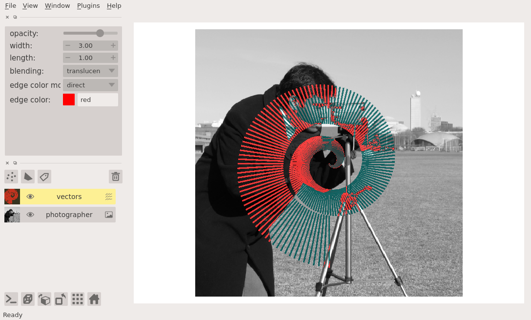
In this example of we will overlay some shapes on the image of a photographer:

%gui qt  # we need to start the Qt event loop before importing napari

ERROR:root:Invalid GUI request 'qt # we need to start the Qt event loop before importing napari', valid ones are:dict_keys(['inline', 'nbagg', 'notebook', 'ipympl', 'widget', None, 'qt4', 'qt', 'qt5', 'wx', 'tk', 'gtk', 'gtk3', 'osx', 'asyncio'])

import napari
import numpy as np
from skimage import data

# create vector data
n = 250
vectors = np.zeros((n, 2, 2), dtype=np.float32)
phi_space = np.linspace(0, 4 * np.pi, n)
radius_space = np.linspace(0, 100, n)
# assign x-y projection
vectors[:, 1, 0] = radius_space * np.cos(phi_space)
vectors[:, 1, 1] = radius_space * np.sin(phi_space)
# assign x-y position
vectors[:, 0] = vectors[:, 1] + 256

# add the image
viewer = napari.view_image(data.camera(), name='photographer')
# add the vectors
viewer.add_vectors(vectors, edge_width=3)

WARNING: QStandardPaths: XDG_RUNTIME_DIR not set, defaulting to '/tmp/runtime-runner'

WARNING:vispy:QStandardPaths: XDG_RUNTIME_DIR not set, defaulting to '/tmp/runtime-runner'

<Vectors layer 'vectors' at 0x7faa896f8b20>

from napari.utils import nbscreenshot

nbscreenshot(viewer)

arguments of view_vectors and add_vectors¶

Both view_vectors and add_vectors have the following doc strings:

napari.view_vectors?

vectors data¶

The input data to the vectors layer must either be a Nx2xD numpy array representing N vectors with start position and projection values in D dimensions, or it must be an N1xN2 … xNDxD, array where each of the first D dimensions corresponds to the voxel of the location of the vector, and the last dimension contains the D values of the projection of that vector. The former representation is useful when you have vectors that can start in arbitrary positions in the canvas. The latter representation is useful when your vectors are defined on a grid, say corresponding to the voxels of an image, and you have one vector per grid.

See here for the example from examples/add_vectors_image.py of a grid of vectors defined over a random image:

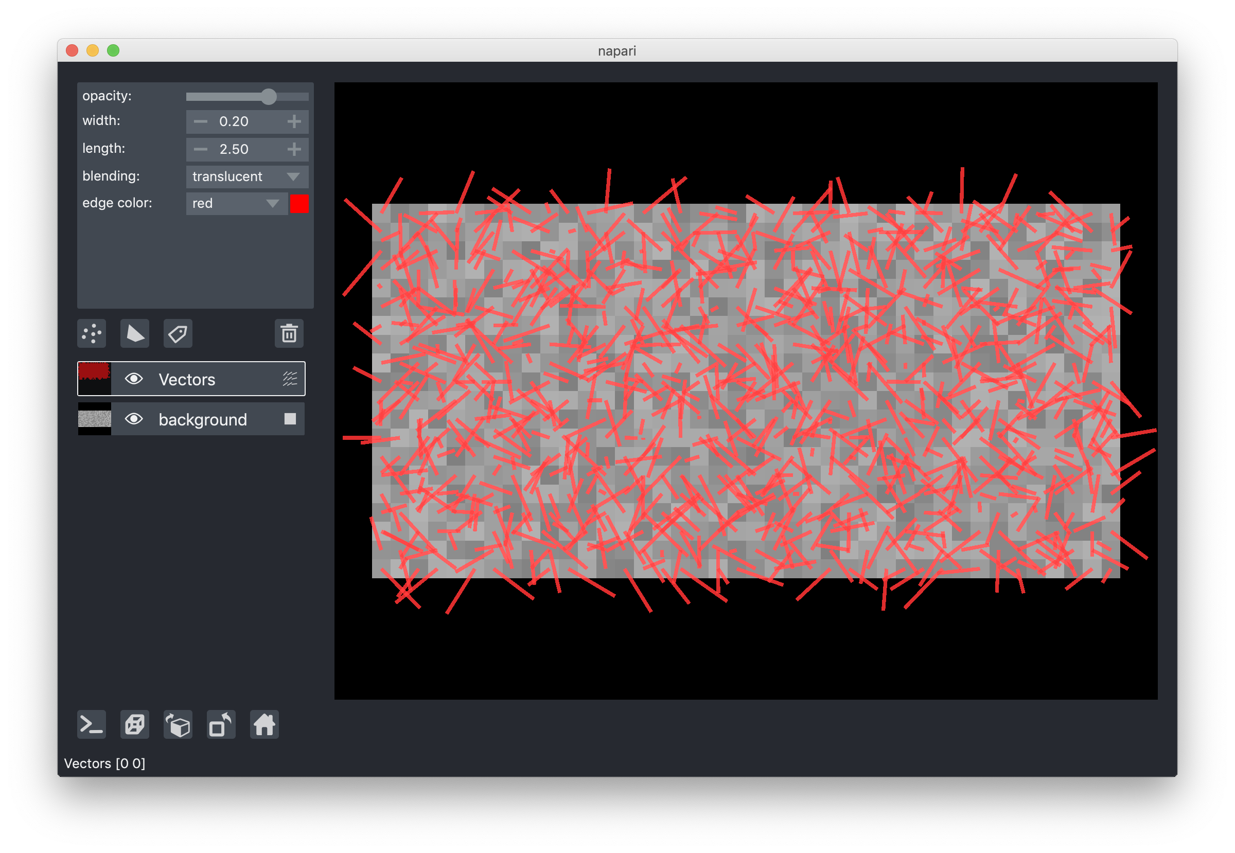
image: add vectors overlaid on an image

Regardless of how the data is passed, we convert it to the Nx2xD representation internally. This representation is accessible through the layer.data property.

Editing the start position of the vectors from the GUI is not possible. Nor is it possible to draw vectors from the GUI. If you want to draw lines from the GUI you should use the Lines shape inside a Shapes layer.

3D rendering of vectors¶

All our layers can be rendered in both 2D and 3D mode, and one of our viewer buttons can toggle between each mode. The number of dimensions sliders will be 2 or 3 less than the total number of dimensions of the layer. See for example the examples/nD_vectors.py to see shapes in both 2D and 3D:

image: nD vectors

changing vector length, width, and color¶

You can multiplicatively scale the length of all the vectors projections using the layer.length property or combobox inside the layer controls panel.

You can also set the width of all the vectors in a layer using the layer.width property or combobox inside the layer controls panel.

You can also set the color of all the vectors in a layer using the layer.edge_color property or dropdown menu inside the layer controls panel.

layer visibility¶

All our layers support a visibility toggle that allows you to set the visible property of each layer. This property is located inside the layer widget in the layers list and is represented by an eye icon.

layer opacity¶

All our layers support an opacity slider and opacity property that allow you to adjust the layer opacity between 0, fully invisible, and 1, fully visible. The opacity value applies globally to all the vectors in the layer.

blending layers¶

All our layers support three blending modes translucent, additive, and opaque that determine how the visuals for this layer get mixed with the visuals from the other layers.

An opaque layer renders all the other layers below it invisible and will fade to black as you decrease its opacity.

The translucent setting will cause the layer to blend with the layers below it if you decrease its opacity but will fully block those layers if its opacity is 1. This is a reasonable default, useful for many applications.

The final blending mode additive will cause the layer to blend with the layers below even when it has full opacity. This mode is especially useful for visualizing multiple layers at the same time.

naming layers¶

All our layers support a name property that can be set inside a text box inside the layer widget in the layers list. The name of each layer is forced into being unique so that you can use the name to index into viewer.layers to retrieve the layer object.

scaling layers¶

All our layers support a scale property and keyword argument that will rescale the layer multiplicatively according to the scale values (one for each dimension). This property can be particularly useful for viewing anisotropic data where the size of the voxel in the z dimension might be different then the size in the x and y dimensions.

translating layers¶

All our layers support a translate property and keyword argument that you can use to offset a layer relative to the other layers, which could be useful if you are trying to overlay two layers for image registration purposes.

layer metadata¶

All our layers also support a metadata property and keyword argument that you can use to store an arbitrary metadata dictionary on the layer.

next steps¶

Hopefully, this tutorial has given you a detailed understanding of the Vectors layer, including how to create one and control its properties. If you’ve explored all the other layer types that napari supports maybe checkout our gallery for some cool examples of using napari with scientific data.